Open in Colab: https://colab.research.google.com/github/casangi/cngi_prototype/blob/master/docs/benchmarking.ipynb
Benchmarks
A demonstration of parallel processing performance of this CNGI prototype against the current released version of CASA using a selection of ALMA datasets representing different computationally demanding configurations and a subset of the VLA CHILES Survey data.
Methodology
Measurement of runtime performance for the component typically dominating compute cost for existing and future workflows – the major cycle – was made against the reference implementation of CASA 6.2. Relevant calls of the CASA task tclean were isolated for direct comparison with the latest version of the cngi-prototype implementation of the mosaic and standard gridders.
The steps of the workflow used to prepare data for testing were:
Download archive data from ALMA Archive
Restore calibrated MeasurementSet using scriptForPI.py with compatible version of CASA
Split off science targets and representative spectral window into a single MeasurementSet
Convert calibrated MeasurementSet into zarr format using
cngi.conversion.convert_ms
This allowed for generation of image data from visibilities for comparison. Tests were run in two different environments:
Dataset Selection
Observations were chosen for their source/observation properties, data volume, and usage mode diversity, particularly the relatively large number of spectral channels, pointings, or executions. Two were observed by the ALMA Compact Array (ACA) of 7m antennas, and two were observed by the main array of 12m antennas.
The datasets from each project code and Member Object Unit Set (MOUS) were processed following publicly documented ALMA archival reprocessing workflows, and come from public observations used used by other teams in previous benchmarking and profiling efforts.
2017.1.00271.S
Compact array observations over many (nine) execution blocks using the mosaic gridder.
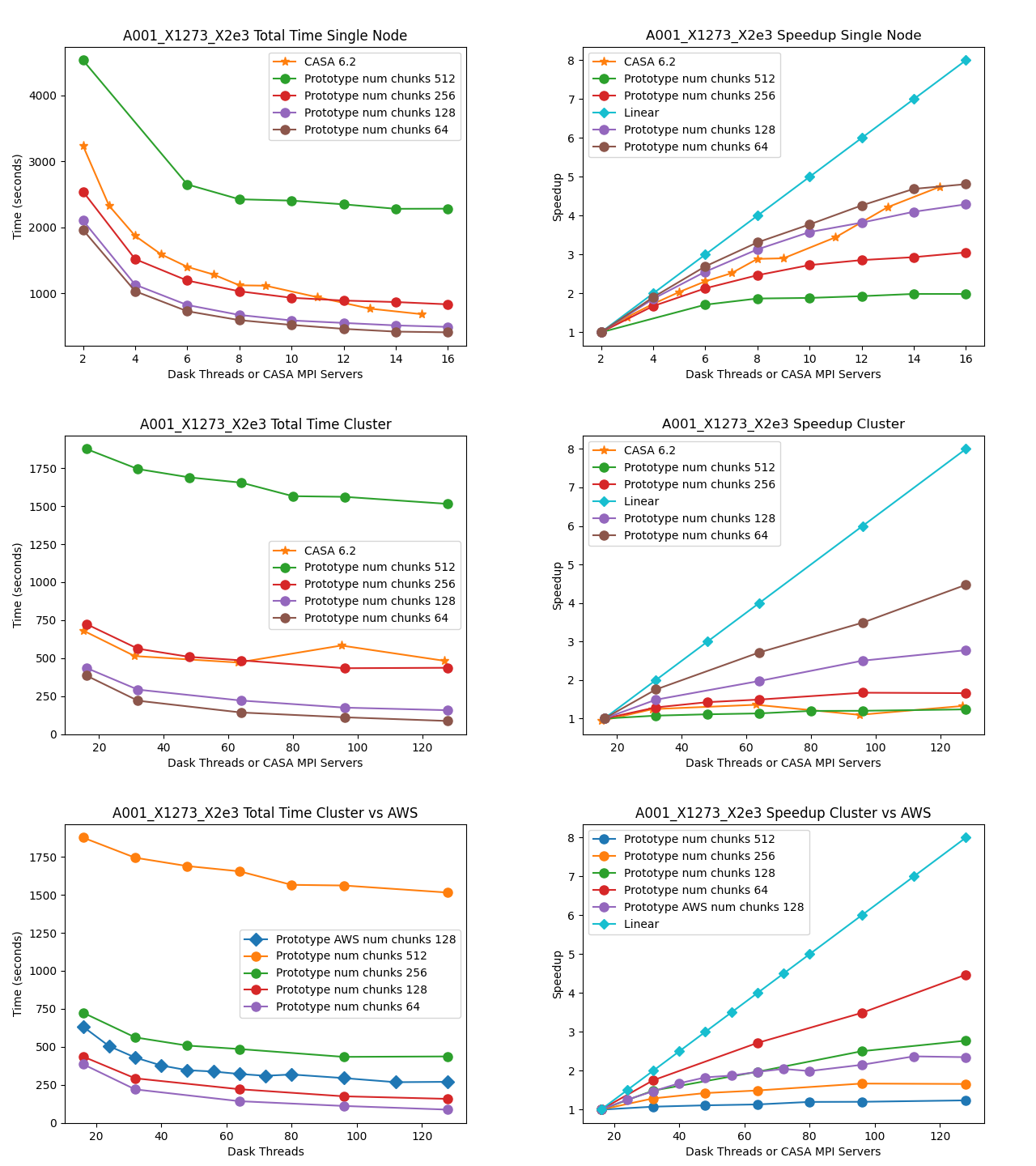
MOUS uid://A001/X1273/X2e3
Measurement Set Rows: 100284
CNGI Shape (time, baseline, chan, pol): (2564, 53, 2048, 2)
Image size (x,y,chan,pol): (400, 500, 2048, 2)
Data Volume (vis.zarr and img.zarr): 30 GB
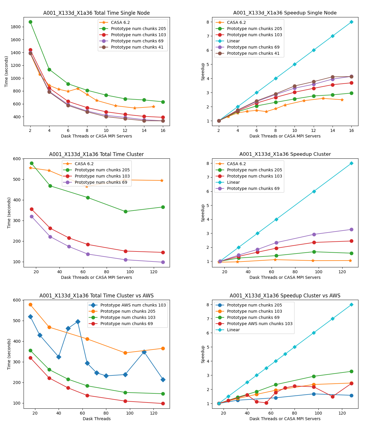
2018.1.01091.S
Compact array observations with many (141) pointings using the mosaic gridder.
MOUS uid://A001/X133d/X1a36
Measurement Set Rows: 31020
CNGI Shape (time, baseline, chan, pol): (564, 55, 1025, 2)
Image size (x,y,chan,pol): (600, 1000, 1025, 2)
Data Volume (vis.zarr and img.zarr): 31 GB
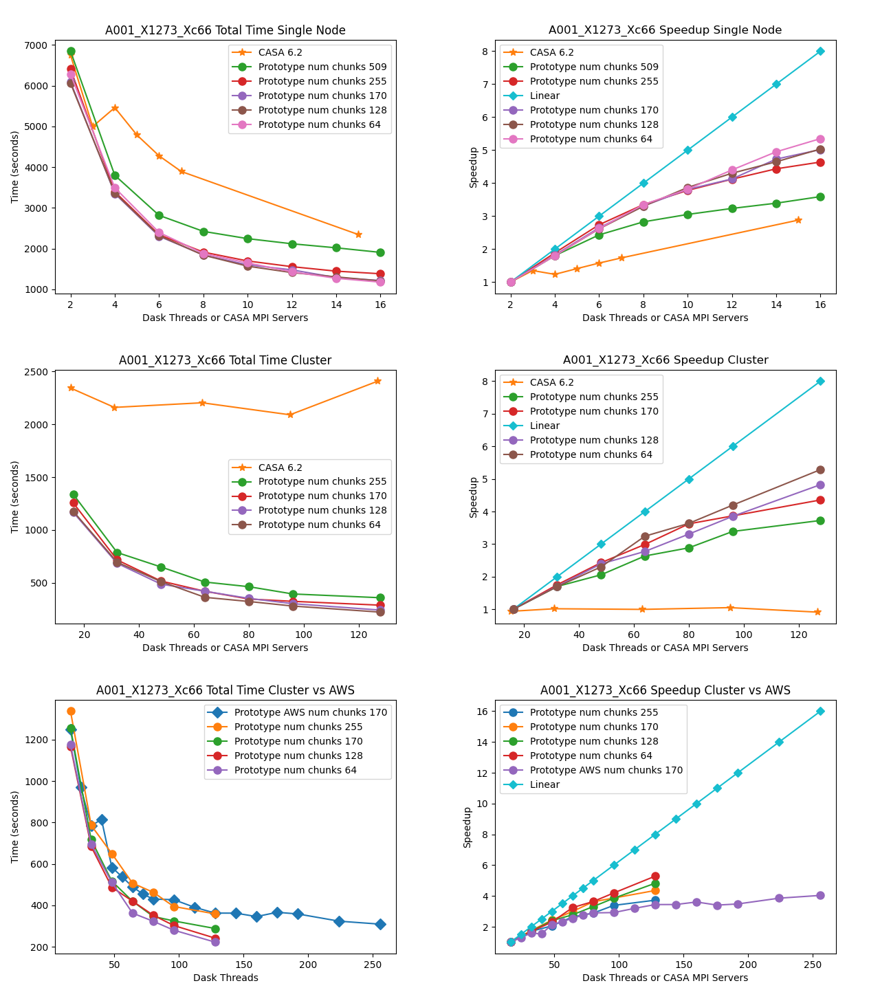
2017.1.00717.S
Main array observations with many spectral channels and visibilities using the standard gridder.
MOUS uid://A001/X1273/Xc66
Measurement Set Rows: 315831
CNGI Shape (time, baseline, chan, pol): (455, 745, 7635, 2)
Image size (x,y,chan,pol): (600, 600, 7635, 2)
Data Volume (vis.zarr and img.zarr): 248 GB
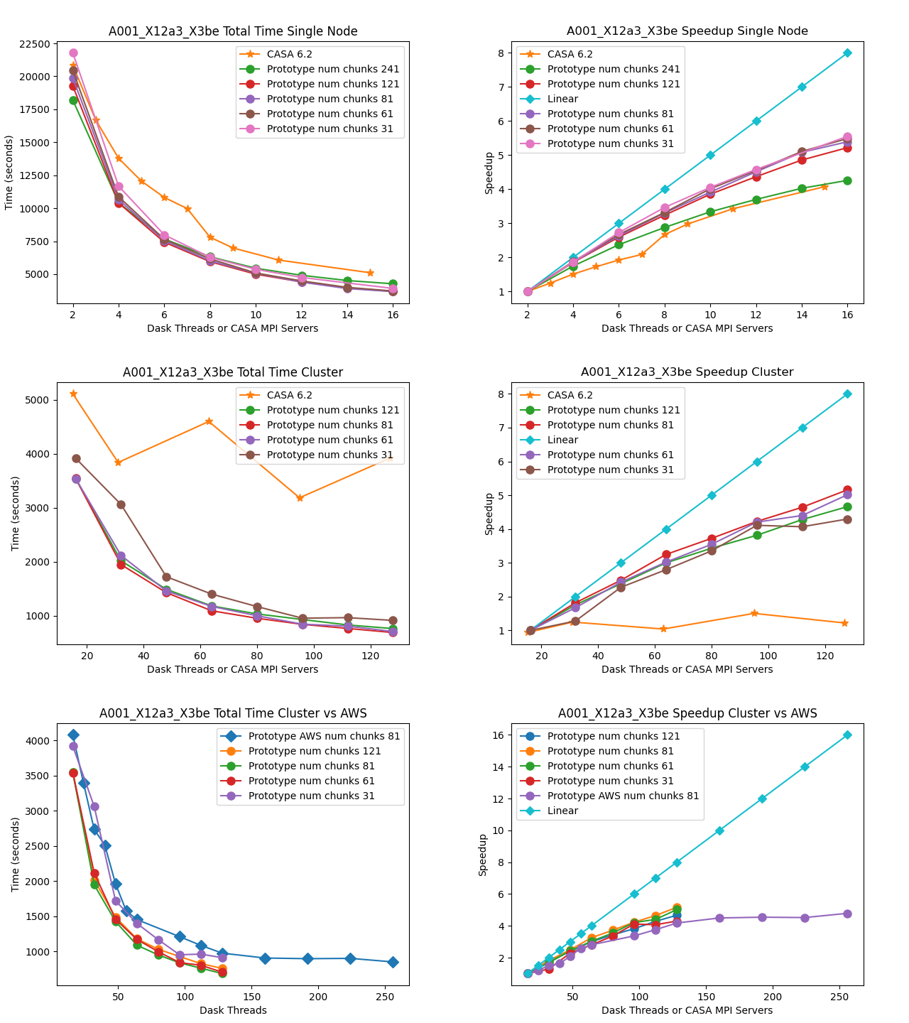
2017.1.00983.S
Main array observations with many spectral channels and visibilities using the mosaic gridder.
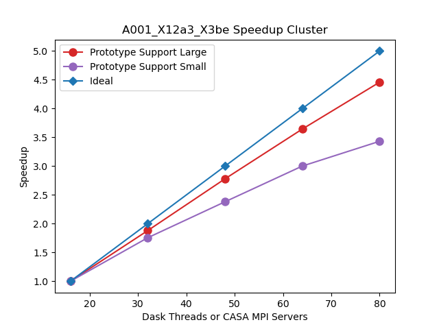
MOUS uid://A001/X12a3/X3be
Measurement Set Rows: 646418
CNGI Shape (time, baseline, chan, pol): (729, 1159, 3853, 2)
Image size (x,y,chan,pol): (1000, 1000, 3853, 2)
Data Volume (vis.zarr and img.zarr): 304 GB
Comparison of Runtimes
Single Machine
The total runtime of the prototype has comparable performance to the CASA 6.2 reference implementations for all datasets. There does not appear to be a performance penalty associated with adopting a pure Python framework compared to the compiled C++/Fortran reference implementation. This is likely due largely to the prototype’s reliance on the numba Just-In-Time (JIT) transpiler, and the C foreign function interface relied on by third-party framework packages including numpy and
scipy.
The Fortran gridding code in CASA is slightly more efficient than the JIT-decorated Python code in the prototype. However, the test implementation more efficiently handles chunked data and does not have intermediate steps where data is written to disk, whereas CASA generates TempLattice files to store intermediate files.
Multi-Node
The total runtime of the prototype mosaic and standard gridders was less than the 6.2 reference implementations except for a couple of suboptimal chunking sizes. For the two larger datasets 2017.1.00717.S and 2017.1.00983.S, a significant speedup of up to six times and ten times, respectively, were achieved. Furthermore, the performance of CASA 6.2 stagnates after a single node because the CASACORE table system can not write the output images to disk in parallel.
Chunking
The chunking of the data determines the number of nodes in Dask graph. As the number of chunks increases, so does scheduler overhead. However, there might not be enough work to occupy all the nodes if there are too few chunks. If data associated with a chunk is too large to fit into memory, the Dask scheduler will spill intermediate data products to disk.
Linear Speedup
Neither CASA nor the prototype achieves a linear speedup due to scheduler overhead, disk io, internode communication, etc. The most computationally expensive step is the gridding of the convolved visibilities onto the uv grid:
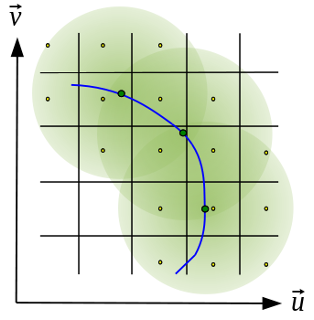
Since the gridding step can be done in parallel, increasing gridding convolution support will increase the part of the work that can be done in parallel. In the figure below, the support size of the gridding convolution kernel is increased from 17x17 to 51x51, consequently, a more linear speedup is achieved.
CHILES Benchmark
The CHILES experiment is an HI large extragalactic survey with over 1000 hours of observing time on the VLA. We choose a subset of the survey data:
Measurement Set Rows: 727272
CNGI Shape (time, baseline, chan, pol): (2072, 351, 30720, 2)
Image size (x,y,chan,pol): (1000, 1000, 30720, 2)
Data Volume (vis.zarr and img.zarr): 2.5 TB
The CHILES dataset has a data volume over 8 times that of the largest ALMA dataset we benchmarked. For an 8 node (128 cores) run, the following results were achieved:
CASA 6.2: 5 hours
Prototype (3840 chunks): 45 minutes ( 6.7 x )
Prototype (256 chunks): 14 hours ( 0.36 x )
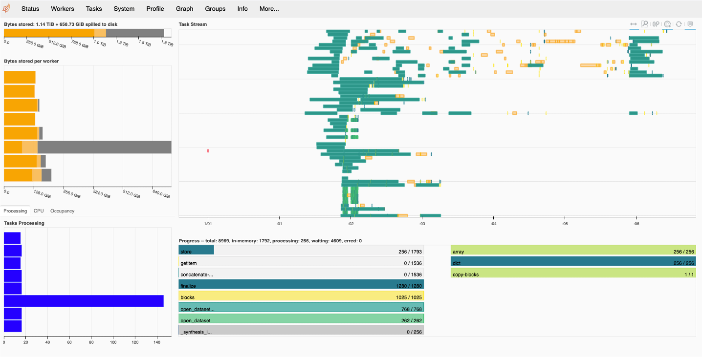
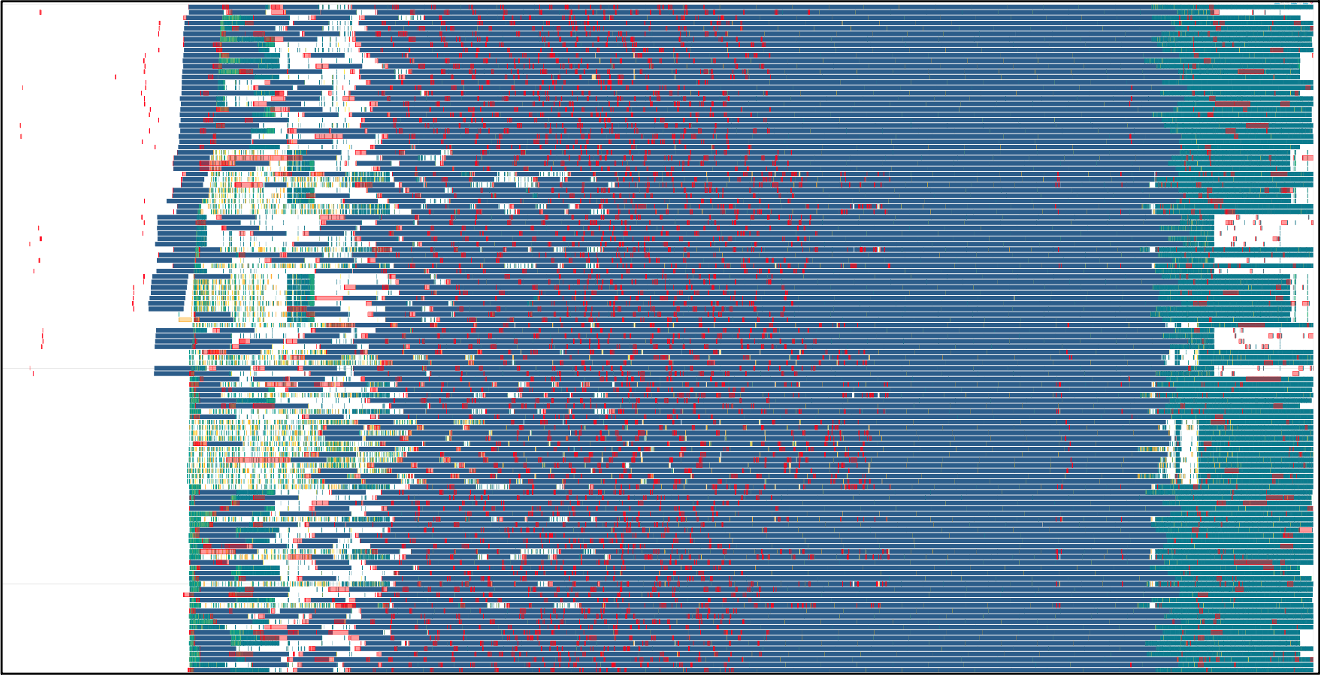
The poor performance of the prototype for 256 chunks is due to the chunks being to large and intermittent data products spilling to disk. This can be seen in the Dask dashboard below (the gray bar shows the data spilled to disk):
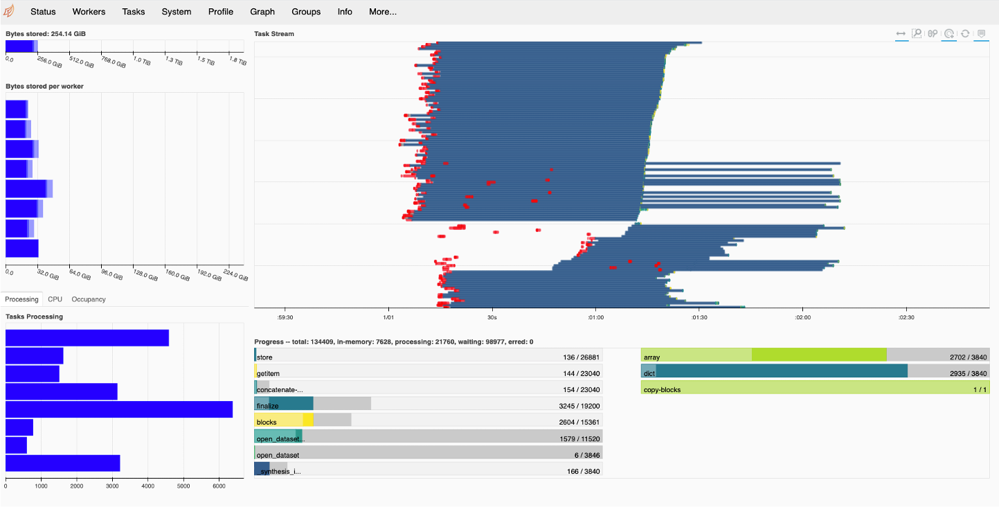
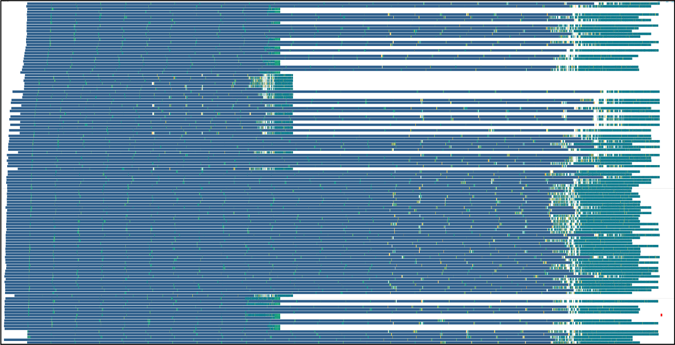
When the number of chunks is increased to 3840, no spilling to disk occurs and the Dask dashboard look like:
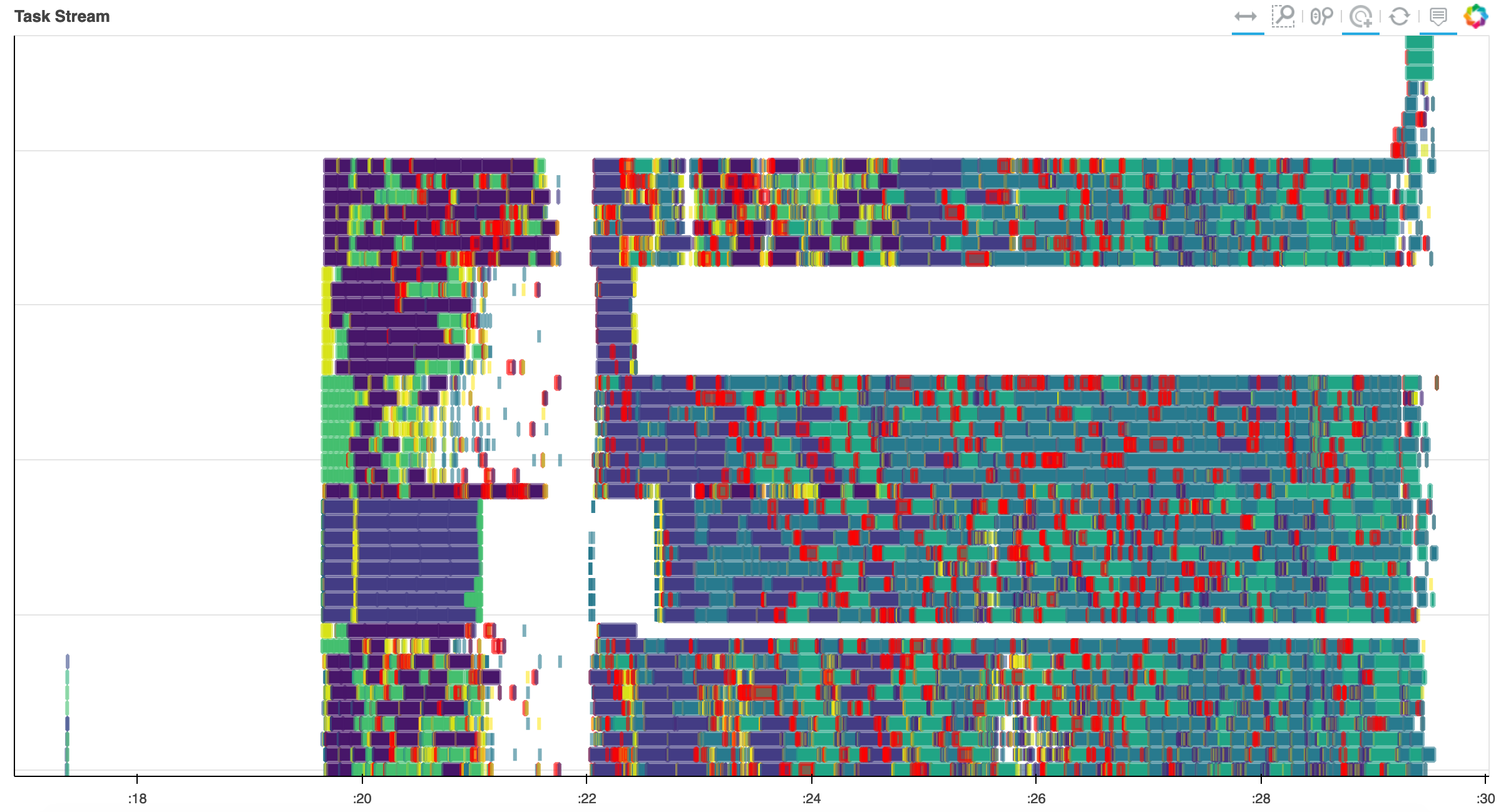
To reduce internode communication overhead, we modified the scheduler with the auto restrictor (AR) plugin developed by Jonathan Kenyon (https://github.com/dask/distributed/pull/4864/files). The first task stream is using the default Dask scheduler, and the communication overhead is shown in red. The second task stream is with the AR plugin enabled. While the communication overhead is eliminated the node work assignment is not balanced. Further modifications of the scheduler will be explored in the future.
Commercial Cloud
The total runtime curves for tests run on AWS show higher variance. One contributing factor that likely dominated this effect was the use of preemptible instances underlying the compute nodes running the worker configuration. For this same reason, some cloud-based test runs show decreased performance with increased scale. This is due to the preemption of nodes and associated redeployment by kubernetes, which sometimes constituted a large fraction of the total test runtime, as demonstrated by the task stream for the following test case. Note the horizontal white bar (signifying to tasks executed) shortly after graph execution begins, as well as some final tasks being assigned to a new node that came online after a few minutes (represented by the new “bar” of 8 rows at top right) in the following figure:
Qualitatively, failure rates were higher during tests of CASA on local HPC infrastructure than they were using dask on the cluster or cloud. The cube refactor shows a noticeable improvement in this area, but still worse than the prototype.
Profiling Results
Benchmarks performed using a single chunk size constitute a test of strong scaling (constant data volume, changing number of processors). Three of the projects used the mosaic gridder, the test of which consisted of multiple function calls composed into a rudimentary “pipeline”. The other project used the standard gridder, with fewer separate function calls and thus relatively more time spent on compute.
The communication of data between workers constituted a relatively small proportion of the total runtime, and the distribution of data between workers was relatively uniform, at all horizontal scalings, with some hot spots beginning to present once tens of nodes were involved. This is demonstrated by the following figure, taken from the performance report of a representative test execution: 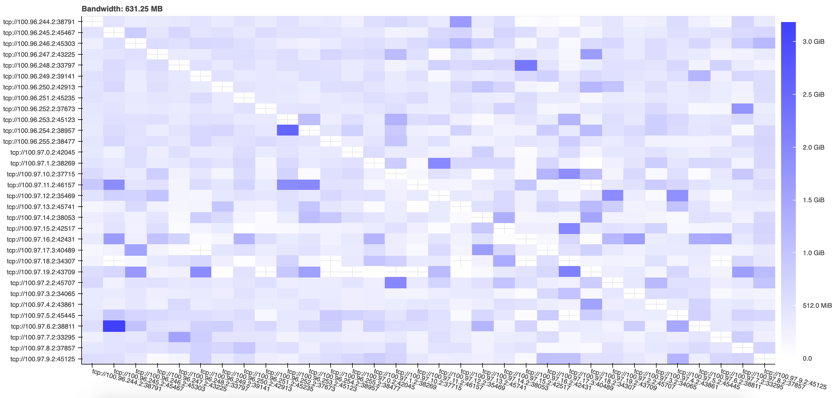
The time overhead associated with graph creation and task scheduling (approximately 100 ms per task for dask) grew as more nodes were introduced until eventually coming to represent a fraction of total execution time comparable to the computation itself, especially in the test cases with smaller data.
Reference Configurations
Dask profiling data were collected using the `performance_report <https://distributed.dask.org/en/latest/diagnosing-performance.html#performance-reports>`__ function in tests run both on-premises and in the commercial cloud.
Some values of the distributed configuration were modified from their defaults:
distributed:
  worker:
    # Fractions of worker memory at which we take action to avoid memory blowup
    # Set any of the lower three values to False to turn off the behavior entirely
    memory:
      target: 0.85  # fraction to stay below (default 0.60)
      spill: 0.92  # fraction at which we spill to disk (default 0.70)
      pause: 0.95  # fraction at which we pause worker threads (default 0.80)
Thread based parallelism in dependent libraries was disabled using environment variables BLAS_NUM_THREADS, BLOSC_NOLOCK, MKL_NUM_THREADS, and OMP_NUM_THREADS.
On-premises HPC cluster
Test execution via Python scripts submitted to Moab scheduler and Torque resource manager with specifications documented internally
Scheduling backend:
dask-jobqueueI/O of visibility and image data via shared infiniband-interconnected lustre file system for access from on-premises high performance compute (HPC) nodes
16 threads per dask worker
Compute via nodes from the cvpost batch queue with Intel(R) Xeon(R) CPU E5-2670 0 @ 2.60GHz with clock speed 1199.865 MHz and cache size 20480 KB.
Commercial cloud (AWS)
Test execution via Jupyter notebooks running on a cloud deployment of the public dask-docker image (version 2021.3.0) backed by a Kubernetes cluster installed with
kops(version 1.18.0), modified to include installation of version 0.0.83 ofcngi-prototypeand associated dependencies.Distributed scheduling backend:
dask.distributedI/O of visibility and image data via Simple Storage Service (S3) object storage for access from commercial cloud Elastic Compute Cloud (EC2) nodes
8 threads per dask worker
Compute via managed Kubernetes cluster backed by a variety of instance types all running on the current daily build of the Ubuntu 20.04 operating system. Cluster coordination service pods were run on a single dedicated
t3.smallinstance. Jupyter notebook, dask scheduler, and etcd service pods were run on a single dedicatedm5dn.4xlargeinstance. Worker pods were run on a configured number of preemptible instances drawn from a pool composed of the following types:m5.4xlarge,m5d.4xlarge,m5dn.4xlarge,r5.4xlarge,r4.4xlarge,m4.4xlarge.
Hyperthreads exposed as vCPUs on the EC2 instances were disabled using the following shell script at instance launch:
spec:
  additionalUserData:
  - content: |
      #!/usr/bin/env bash
      for cpunum in $(cat /sys/devices/system/cpu/cpu*/topology/thread_siblings_list | cut -s -d, -f2- | tr ',' '\n' | sort -un)
      do
        echo 0 > /sys/devices/system/cpu/cpu$cpunum/online
      done
    name: disable_hyperthreading.sh
    type: text/x-shellscript
  image: