Open in Colab: https://colab.research.google.com/github/casangi/cngi_prototype/blob/master/docs/development.ipynb
Development
READ THIS BEFORE YOU CONTRIBUTE CODE!!!
Organization
The CNGI Prototype is organized into packages and modules as described below. Base infrastructure, data manipulation and mathematics are contained in the CNGI package. Higher level data reduction functionality is contained in the ngCASA package. Within each package are a set of modules, with each module responsible for a different functional area.
CNGI package
conversion : convert legacy CASA data files to CNGI compatible files
dio : data objects to/from CNGI compatible data files
vis : operations on visibility data objects
image : operations on image data objects
direct : access/initialize the underlying parallel processing framework
ngCASA package
flagging : Generates flags for visibility data.
calibration : Generates and applies calibration solutions to visibility data.
imaging : Converts visibility data to images and applies antenna primary beam and w-term corrections.
deconvolution : Deconvolves PSF from images and combines images.
The cngi_prototype repository on GitHub contains both packages along with supporting folders docs and tests.
Architecture
The CNGI Prototype application programming interface (API) is a set of flat, stateless functions that take an xarray Dataset as an input parameter and return a new xarray Dataset (XDS) as output. The term “flat” means that the functions are not allowed to call each other, and the term “stateless” means that they may not access any global data outside the parameter list, nor maintain any persistent internal data.
The CNGI Prototype code base is not object oriented, and instead follows a more functional paradigm. Objects are indeed used to hold Visibility and Image data, but they come directly from the underlying xarray/dask framework and are not extended in any way.
The data variables in the XDS are associated with task graphs. Compute is only triggered when the user explicitly calls compute on the XDS or instructs a function to save to disk.
The CNGI Prototype adheres to a strict design philosophy with the following RULES:
Each file in a module must have exactly one function exposed to the external API (by docstring and __init__.py).
The exposed function name should match the file name.
Must use stateless functions, not classes.
Files in a module cannot import each other.
Files in separate modules cannot import each other.
Special _utility modules may exist for internal functions meant to be shared across modules/files. But each module file should be as self contained as possible.
A module’s utility files may only be imported by that module’s API files.
A package’s utility files may only be imported by other modules in that package.
No utility functions may be exposed to the external API.
cngi_prototype
|-- cngi
|    |-- module1
|    |     |-- __init__.py
|    |     |-- file1.py
|    |     |-- file2.py
|    |     | ...
|    |-- module2
|    |     |-- __init__.py
|    |     |-- file3.py
|    |     |-- file4.py
|    |     | ...
|    |-- _utils
|    |     |-- __init__.py
|    |     |-- _file5.py
|    |     |-- _file6.py
|    |     | ...
|    | ...
|-- ngcasa
|    |-- module1
|    |     |-- __init__.py
|    |     |-- file1.py
|    |     |-- file2.py
|    |     | ...
|    |     |-- _module1_utils
|    |     |     |-- __init__.py
|    |     |     |-- _check_module1_parms.py
|    |     |     |-- _file5.py
|    |     |     |-- _file6.py
|    |     |     | ...
|    |-- module2
|    |     |-- __init__.py
|    |     |-- file3.py
|    |     |-- file4.py
|    |     | ...
|    |     |-- _module2_utils
|    |     |     |-- __init__.py
|    |     |     |-- _check_module2_parms.py
|    |     |     |-- _file7.py
|    |     |     |-- _file8.py
|    |     |     | ...
|    | ...
|-- docs
|    | ...
|-- tests
|    | ...
|-- requirements.txt
|-- setup.py
File1, file2, file3 and file4 MUST be documented in the API exactly as they appear. They must NOT import each other. _file5 and _file6 are utility files, they must NOT be documented in the API. They may be imported by file1-4 (cngi package) and file1-2 (ngcasa package).
There are several important files to be aware of:
__init__.py : dictates what is seen by the API and importable by other functions
requirements.txt : lists all library dependencies for development, used by IDE during setup
setup.py : defines how to package the code for pip, including version number and library dependencies for installation
**_check_module_parms.py** : Each module has a _check_module_parms.py file that has functions that check the input parameters of the module’s API functions. The parameter defaults are also defined here.
**_check_parms.py** : Provides the _check_parms and _check_storage_parms functions. The _check_parms is used by all the _check_module_parms.py files to check parameter data types, values and set defaults. The storage_parm is parameter that is common to all API functions is checked by _check_storage_parms.
**_store.py** : Provides the _store function that stores datasets or appends data variables. All API functions use this function.
CNGI Function Template
def myfunction(xds, param_1, ..., param_m):
    """
    Description of function

    Parameters
    ----------
    xds : xarray.core.dataset.Dataset
       input xarray dataset
    param_1 : type
       description of this parameter
    ...
    parms_n : type
       description of this parameter

    Returns
    -------
    xarray.core.dataset.Dataset
       new output xarray dataset
    """

    ### Import Statements
    import numpy as np
    ...

    ### Parameter Checking
    assert(param_1 == what_it_shoud, "ERROR: param_1 is wrong")
    ...

    ### Function code
    c = xds.a + xds.b
    ...

    ### Return a new xds, leaving input untouched
    nxds = xds.assign({'mynewthing':c}

    return nxds
By default calling an CNGI function will not do computation, but rather build a graph of the computation (example of a graph). Computation can be triggered by using dask.compute(dataset).
Data Structures
Data is stored in Zarr files with Xarray formatting (which is specified in the metadata). The data is stored as N-dimensional arrays that can be chunked on any axis. The ngCASA/CNGI data formats are:
vis.zarr Visibility data (measurement set).
img.zarr Images (also used for convolution function cache).
cal.zarr Calibration tables.
tel.zar Telescope layout (used for simulations)
Other formats will be added as needed.
CNGI will provide functions to convert between the new Zarr formats and legacy formats (such as the measurement set, FITS files, ASDM, etc.). The current implementations of the Zarr formats are not fully developed and are only sufficient for prototype development.
Zarr data formats rules:
Data variable names are always uppercase and dimension coordinates are lowercase.
Data variable names are not fixed but defaults exist, for example the data variable that contains the uvw data default name is UVW. This flexibility allows for the easy inclusion of more advanced algorithms (for example multi-term deconvolution that produces Taylor term images).
Dimension coordinates and coordinates have fixed names.
Dimension coordinates are not chunked.
Data variables and coordinates are chunked and should have consistent chunking with each other.
Any number of data variables can be in a dataset but must share a common coordinate and chunking system.
Framework
The abstraction layers of ngCASA and CNGI are unified by the paradigm of functional programming:
Build a directed acyclic graph (DAG) of blocked algorithms composed from functions (the edges) and data (the vertices) for lazy evaluation by a scheduler process coordinating a network of (optionally distributed and heterogeneous) machine resources.
This approach relies on three compatible packages to form the core of the framework:
Dask’s specificiation of the DAG coordinates processing and network resources
Zarr’s specification of blocked data structures coordinates input/output and serialization resources
Xarray’s specficiation of multidimensional indexed arrays serves as the in-memory representation and interface to the other components of the framework
The relationship between these libraries can be conceptualized by the following diagram:
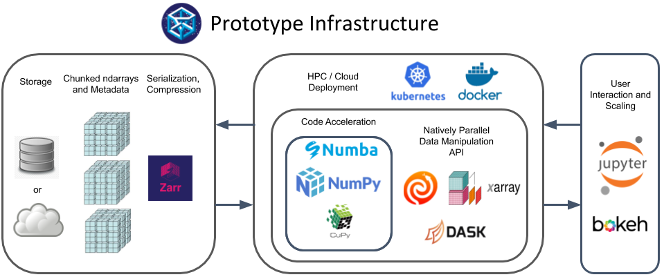
In the framework data is stored in the Zarr format in a file mounted on a local disk or in the cloud. The Dask scheduler manages N worker processes identified to the central scheduler by their unique network address and coordinating M threads. Each thread applies functions to a set of data chunks. Xarray wraps Dask functions and labels the Dask arrays for ease of interface. Any code that is wrapped with Python can be parallelized with Dask. Therefore, the option to use C++, Numba or other custom high performance computing (HPC) code is retained. The size of the Zarr data chunks (on disk) and Dask data chunks do not have to be the same, this is further explained in the chunking section. Data chunks can either be read from disk as they are needed for computation or the data can be persisted into memory.
Dask and Dask Distributed
Dask is a flexible library for parallel computing in Python and Dask Distributed provides a centrally managed, distributed, dynamic task scheduler. A Dask task graph describes how tasks will be executed in parallel. The nodes in a task graph are made of Dask collections. Different Dask collections can be used in the same task graph. For the CNGI and ngCASA projects Dask array and Dask delayed collections will
predominantly be used. Explanations from the Dask website about Dask arrays and Dask delayed:
Dask array implements a subset of the NumPy ndarray interface using blocked algorithms, cutting up the large array into many small arrays. This lets us compute on arrays larger than memory using all of our cores. We coordinate these blocked algorithms using Dask graphs.
Sometimes problems don’t fit into one of the collections like dask.array or dask.dataframe. In these cases, users can parallelize custom algorithms using the simpler dask.delayed interface. This allows one to create graphs directly with a light annotation of normal python code.
The following diagram taken from the Dask website illustrates the components of the chosen parallelism framework.

Dask/Dask Distributed Advantages:
Parallelism can be achieved over any dimension, since it is determined by the data chunking.
Data can either be persisted into memory or read from disk as needed. As processing is finished chunks can be saved. This enables the processing of data that is larger than memory.
Graphs can easily be combined with
dask.compute()to concurrently execute multiple functions in parallel. For example a cube and continuum image can be created in parallel.
Xarray
Xarray provides N-Dimensional labeled arrays and datasets in Python. The Xarray dataset is used to organize and label related arrays. The Xarray website gives the following definition of a dataset:
“xarray.Dataset is Xarray’s multi-dimensional equivalent of a DataFrame. It is a dict-like container of labeled arrays (DataArray objects) with aligned dimensions.”
The Zarr disk format and Xarray dataset specification are compatible if the Xarray to_zarr and open_zarr functions are used. The compatibility is achieved by requiring the Zarr group to have labeling information in the metadata files and a depth of one (see the Zarr section for further explanation).
When xarray.open_zarr(zarr_group_file) is used the array data is not loaded to memory (there is a parameter to force this), rather the metadata is loaded and a lazy loaded Xarray dataset is created. For example a dataset that consists of three dimension coordinates (dim_), two coordinates (coord_) and three data variables (Data_) would have the following structure (this is what is displayed if a print command is used on a lazy loaded dataset):
<xarray.Dataset>
Dimensions:        (dim_1: d1, dim_2: d2, dim_3: d3)
Coordinates:
    coord_1      (dim_1) data_type_coord_1 dask.array<chunksize=(chunk_d1,), meta=np.ndarray>
    coord_2      (dim_1, dim_2)  data_type_coord_2 dask.array<chunksize=(chunk_d1,chunk_d2), meta=np.ndarray>
  * dim_1        (dim_1) data_type_dim_1 np.array([x_1, x_2, ..., x_d1])
  * dim_2        (dim_2) data_type_dim_2 np.array([y_1, y_2, ..., y_d2])
  * dim_3        (dim_3) data_type_dim_3 np.array([z_1, z_2, ..., z_d3])

Data variables:
    DATA_1       (dim2) data_type_DATA_1 dask.array<chunksize=(chunk_d2,), meta=np.ndarray>
    DATA_2       (dim1) data_type_DATA_2 dask.array<chunksize=(chunk_d1,), meta=np.ndarray>
    DATA_3       (dim1,dim2,dim3) data_type_DATA_3 dask.array<chunksize=(chunk_d1,chunk_d2,chunk_d3), meta=np.ndarray>

Attributes:
    attr_1:        a1
    attr_2:        a2
d1, d2, d3 are integers.
a1, a2 can be any data type that can be stored in a JSON file.
data_type_dim_, data_type_coord_ , data_type_DATA_ can be any acceptable NumPy array data type.
Explanations of dimension coordinates, coordinates and data variables from the Xarray website:
dim_ “Dimension coordinates are one dimensional coordinates with a name equal to their sole dimension (marked by * when printing a dataset or data array). They are used for label based indexing and alignment, like the index found on a pandas DataFrame or Series. Indeed, these dimension coordinates use a pandas. Index internally to store their values.”
coord_ “Coordinates (non-dimension) are variables that contain coordinate data, but are not a dimension coordinate. They can be multidimensional (see Working with Multidimensional Coordinates), and there is no relationship between the name of a non-dimension coordinate and the name(s) of its dimension(s). Non-dimension coordinates can be useful for indexing or plotting; otherwise, xarray does not make any direct use of the values associated with them. They are not used for alignment or automatic indexing, nor are they required to match when doing arithmetic.”
DATA_ The array that dimension coordinates and coordinates label.
Zarr
Data is stored in Zarr files with Xarray formatting (which is specified in the metadata). The data is stored as N-dimensional arrays that can be chunked on any axis. The ngCASA/CNGI data formats are:
vis.zarr Visibility data (measurement set).
img.zarr Images (also used for convolution function cache).
cal.zarr Calibration tables.
tel.zar Telescope layout (used for simulations)
Other formats will be added as needed.
CNGI will provide functions to convert between the new Zarr formats and legacy formats (such as the measurement set, FITS files, ASDM, etc.). The current implementations of the Zarr formats are not fully developed and are only sufficient for prototype development.
Zarr data formats rules:
Data variable names are always uppercase and dimension coordinates are lowercase.
Data variable names are not fixed but defaults exist, for example the data variable that contains the uvw data default name is UVW. This flexibility allows for the easy inclusion of more advanced algorithms (for example multi-term deconvolution that produces Taylor term images).
Dimension coordinates and coordinates have fixed names.
Dimension coordinates are not chunked.
Data variables and coordinates are chunked and should have consistent chunking with each other.
Any number of data variables can be in a dataset but must share a common coordinate and chunking system.
Zarr is the chosen data storage library for the CNGI Prototype. It provides an implementation of chunked, compressed, N-dimensional arrays that can be stored on disk, in memory, in cloud-based object storage services such as Amazon S3, or any other collection that supports the MutableMapping interface.
Compressed arrays can be hierarchically organized into labeled groups. For the CNGI Prototype, the Zarr group hierarchy is structured to be compatible with the Xarray dataset convention (a Zarr group contains all the data for an Xarray dataset):
My/Zarr/Group
    |-- .zattrs
    |-- .zgroup
    |-- .zmetadata

    |-- Array_1
    |    |-- .zattrs
    |    |-- .zarray
    |    |-- 0.0.0. ... 0
    |    |-- ...
    |    |-- C_1.C_2.C_3. ... C_D
    |-- ...
    |-- Array_N_c
    |    |-- ...
The group is accessed by a logical storage path (in this case, the string My/Zarr/Group) and is self-describing; it contains metadata in the form of hidden files (.zattrs, .zgroup and .zmetadata ) and a collection of folders. Each folder contains the data for a single array along with two hidden metadata files (.zattrs, .zarray). The metadata files are used to create the lazily loaded representation of the dataset (only metadata is loaded). The data of each array is
chunked and stored in the format x_1,x_2,x_3, ..., x_D where D is the number of dimensions and x_i is the chunk index for the ith dimension. For example a three dimensional array with two chunks in the first dimension and three chunks in the second dimension would consist of the following files 0.0.0, 1.0.0, 0.1.0, 1.1.0, 0.2.0, 1.2.0.
Group folder metadata files (encoded using JSON):
.zgroupcontains an integer defining the version of the storage specification. For example:{ "zarr_format": 2 }.zattrsdescribes data attributes that can not be stored in an array (this file can be empty). For example:{ "append_zarr_time": 1.8485729694366455, "auto_correlations": 0, "ddi": 0, "freq_group": 0, "ref_frequency": 372520022603.63745, "total_bandwidth": 234366781.0546875 }.zmetadatacontains all the metadata from all other metadata files (both in the group directory and array subdirectories). This file does not have to exist, however it can decrease the time it takes to create the lazy loaded representation of the dataset, since each metadata file does not have to be opened and read separately. If any of the files are changed or files are added the.zmetadatafile must be updated withzarr.consolidate_metadata(group_folder_name).
Array folder metadata files (encoded using JSON):
.zarraydescribes the data: how it is chunked, the compression used and array properties. For example the.zarrayfile for a DATA array (contains the visibility data) would contain:{ "chunks": [270,210,12,1], "compressor": {"blocksize": 0,"clevel": 2,"cname": "zstd","id": "blosc","shuffle": 0}, "dtype": "<c16", "fill_value": null, "filters": null, "order": "C", "shape": [270,210,384,1], "zarr_format": 2 }Zarr supports all the compression algorithms implemented in numcodecs (‘zstd’, ‘blosclz’, ‘lz4’, ‘lz4hc’, ‘zlib’, ‘snappy’).
.zattrsis used to label the arrays so that an Xarray dataset can be created. The labeling creates three types of arrays:Dimension coordinates are one dimensional arrays that are used for label based indexing and alignment of data variable arrays. The array name is the same as its sole dimension. For example the
.zattrsfile in the “chan” array would contain:{ "_ARRAY_DIMENSIONS": ["chan"] }Coordinates can have any number of dimensions and are a function of dimension coordinates. For example the “declination” coordinate is a function of the d0 and d1 dimension coordinates and its
.zattrsfile contains:{ "_ARRAY_DIMENSIONS": ["d0","d1"] }Data variables contain the data that dimension coordinates and coordinates label. For example the DATA data variable’s
.zattrsfile contains:{ "_ARRAY_DIMENSIONS": ["time","baseline","chan","pol"], "coordinates": "interval scan field state processor observation" }
Zarr Advantages:
Designed for concurrency, compatible out-of-the-box with chosen parallelism framework (Dask).
Wide variety of compression algorithms supported, see numcodecs. Each data variable can be compressed using a different compression algorithm.
Supports chunking along any dimension.
Has a defined cloud interface.
Chunking
In the zarr and dask model, data is broken up into chunks to improve efficiency by reducing communication and increasing data locality. The zarr chunk size is specified at creation or when converting from CASA6 format datasets. The Dask chunk size can be specified in the cngi.dio.read_vis and cngi.dio.read_image calls using the chunks parameter. The dask and zarr chunking do not have to be the same. The zarr chunking is what
is used on disk and the dask chunking is used during parallel computation. However, it is more efficient for the dask chunk size to be equal to or a multiple of the zarr chunk size (to stop multiple reads of the same data). This hierarchy of chunking allows for flexible and efficient algorithm development. For example cube imaging is more memory efficient if chunking is along the channel axis (the
benchmarking example demonstrates this). Note, chunking can be done in any combination of dimensions.
Numba
Numba is an open source JIT (Just In Time) compiler that uses LLVMto translate a subset of Python and NumPy code into fast machine code from a chain of intermediate representations. Numba is used in ngCASA for functions that have long nested for loops (for example the gridder code). Numba can be used by adding the @jit decorator above a function:
@jit(nopython=True, cache=True, nogil=True)
def my_func(input_parms):
    does something ...
Explanation of jit arguments from the Numba:
nopython: > The behaviour of the nopython compilation mode is to essentially compile the decorated function so that it will run entirely without the involvement of the Python interpreter. This is the recommended and best-practice way to use the Numba jit decorator as it leads to the best performance.
cache: > To avoid compilation times each time you invoke a Python program, you can instruct Numba to write the result of function compilation into a file-based cache.
nogil: > Whenever Numba optimizes Python code to native code that only works on native types and variables (rather than Python objects), it is not necessary anymore to hold Python’s global interpreter lock (GIL)”
A 5 minute guide to starting with Numba can be found here.
Numba also has functionality to run code on CUDA and AMD ROC) GPUs. This will be explored in the future.
Parallel Code with Dask
Code can be parallelized in three different ways:
Built in Dask array functions. The list of dask.array functions can be found here. For example the fast Fourier transform is a built in parallel function:
uncorrected_dirty_image = dafft.fftshift(dafft.ifft2(dafft.ifftshift(grids_and_sum_weights[0], axes=(0, 1)),
                                                     axes=(0,1)), axes=(0, 1))
Apply a custom function to each Dask data chunk. There are numerous Dask functions, with varying capabilities, that do this: map_blocks, map_overlap, apply_gufunc, blockwise. For example the
dask.map_blockfunction is used to divide each image in a channel with the gridding convolutional kernel:
def correct_image(uncorrected_dirty_image, sum_weights, correcting_cgk):
    sum_weights[sum_weights == 0] = 1
    corrected_image = (uncorrected_dirty_image / sum_weights[None, None, :, :])
        / correcting_cgk[:, :, None, None]
    return corrected_image

corrected_dirty_image = dask.map_blocks(correct_image, uncorrected_dirty_image,
                                      grids_and_sum_weights[1],correcting_cgk_image)
Custom parallel functions can be built using dask.delayed objects. Any function or object can be delayed. For example the gridder is implemented using dask.delayed:
for c_time, c_baseline, c_chan, c_pol in iter_chunks_indx:
    sub_grid_and_sum_weights = dask.delayed(_standard_grid_numpy_wrap)(
    vis_dataset[grid_parms["data_name"]].data.partitions[c_time, c_baseline, c_chan, c_pol],
    vis_dataset[grid_parms["uvw_name"]].data.partitions[c_time, c_baseline, 0],
    vis_dataset[grid_parms["imaging_weight_name"]].data.partitions[c_time, c_baseline, c_chan, c_pol],
    freq_chan.partitions[c_chan],
    dask.delayed(cgk_1D), dask.delayed(grid_parms))
    grid_dtype = np.complex128
Documentation
All CNGI documentation is automatically rendered from files placed in the docs folder using the Sphinx tool. A Readthedocs service scans for updates to the Github repository and automatically calls Sphinx to build new documentation as necessary. The resulting documentation html is hosted by readthedocs as a CNGI website.

Compatible file types in the docs folder that can be rendered by Sphinx include:
Markdown (.md)
reStructuredText (.rst)
Jupyter notebook (.ipynb)
Sphinx extension modules are used to automatically crawl the cngi code directories and pull out function definitions. These definitions end up in the API section of the documentation. All CNGI functions must conform to the numpy docstring format.
The nbsphinx extension module is used to render Jupyter notebooks to html.
IDE
The CNGI team recommends the use of the PyCharm IDE for developing CNGI code. PyCharm provides a simple (relatively) unified environment that includes Github integration, code editor, python shell, system terminal, and venv setup.

CNGI also relies heavily on Google Colaboratory for both documentation and code execution examples. Google colab notebooks integrate with Github and allow markdown-style documentation interleaved with executable python code. Even in cases where no code is necessary, colab notebooks are the preferred choice for markdown documentation. This allows other team members to make documentation updates in a simple, direct manner.

PyPi Packages
CNGI is distributed and installed via pip by hosting packages on pypi. The pypi test server is available to all authorized CNGI developers to upload an evaluate their code branches.
![]()
Typically, the Colab notebook documentation and examples will need a pip installation of CNGI to draw upon. The pypi test server allows notebook documentation to temporarily draw from development branches until everything is finalized in a Github pull request and production pypi distribution.
Developers should create a .pypirc file in their home directory for convenient uploading of distributions to the pip test server. It should look something like:
[distutils]
index-servers =
     pypi
     pypitest

[pypi]
username = yourusername
password = yourpassword

[pypitest]
repository = https://test.pypi.org/legacy/
username = yourusername
password = yourpassword
Production packages are uploaded to the main pypi server by a subset of authorized CNGI developers when a particular version is ready for distribution.
Step by Step
Concise steps for contributing code to CNGI
Install IDE
Request that your Github account be added to the contributors of the CNGI repository
Make sure Python 3.6 and Git are installed on your machine
Download and install the free PyCharm Community edition. On Linux, it is just a tar file. Expand it and execute pycharm.sh in the bin folder via something like:
$ ./pycharm-community-2020.1/bin/pycharm.sh
From the welcome screen, click
Get from Version ControlAdd your Github account credentials to PyCharm and then you should see a list of all repositories you have access to
Select the CNGI repository and set an appropriate folder location/name. Click “Clone”.
Go to:
File -> Settings -> Project: xyz -> Python Intrepreter
and click the little cog to add a new Project Interpreter. Make a new Virtualenv environment, with the location set to a venv subfolder in the project directory. Make sure to use Python 3.6.
Double click the
requirements.txtfile that was part of the git clone to open it in the editor. That should prompt PyCharm to ask you if you want to “Install requirements” found in this file. Yes, you do. You can ignore the stuff about plugins.All necessary supporting Python libraries will now be installed in to the venv created for this project (isolating them from your base system). Do NOT add any project settings to Git.
Develop stuff
Double click on files to open in editor and make changes.
Create new files with:
right-click -> New
Move / rename / delete files with:
right-click -> Refactor
Run code interactively by selecting “Python Console” from the bottom of the screen. This is your venv enviornment with everything from requirements.txt installed in addition to the cngi package. You can do things like this:
>>> from cngi.dio import read_vis
>>> xds = read_vis('path\to\data.vis.zarr')
When you make changes to a module (lets say read_vis for example), close the Python Console and re-open it, then import the module again to see the changes.
Commit changes to your local branch with
right-click -> Git -> Commit File
Merge latest version of Github master trunk to your local branch with
right-click -> Git -> Repository -> Pull
Push your local branch up to the Github master trunk with
right-click -> Git -> Repository -> Push
Make a Pip Package
If not already done, create an account on pip (and the test server) and have a CNGI team member grant access to the package. Then create a
.pypircfile in your home directory.Set a unique version number in
setup.pyby using the release candidate label, as in:version='0.0.48rc1'
Build the source distribution by executing the following commands in the PyCharm Terminal (button at the bottom left):
$ rm -fr dist
$ python setup.py sdist
call twine to upload the sdist package to pypi-test:
$ python -m twine upload dist/* -r pypitest
Enjoy your pip package as you would a real production one by pointing to the test server:
$ pip install --extra-index-url https://test.pypi.org/simple/ cngi-prototype==0.0.48rc1
Update the Documentation
A bulk of the documentation is in the
docsfolder and in the ‘.ipynb’ format. These files are visible through PyCharm, but should be edited and saved in Google Colab. The easiest way to do this is not navigate to the Github docs folder and click on the .ipynb file you want to edit. There is usually anopen in colablink at the top.Alternatively, notebooks can be accessed in Colab by combining a link prefix with the name of the .ipynb file in the repository
docsfolder. For example, this page you are reading now can be edited by combining the colab prefix:https://colab.research.google.com/github/casangi/cngi_prototype/blob/master/docs/
with the filename of this notebook:
development.ipynb
producing a link of: https://colab.research.google.com/github/casangi/cngi_prototype/blob/master/docs/development.ipynb
In Colab, make the desired changes and then select
File -> Save a copy in Github
enter you Github credentials if not already stored with Google, and then select the CNGI repository and the appropriate path/filename, i.e.
docs/development.ipynbReadthedocs will detect changes to the Github master and automatically rebuild the documentation hosted on their server (this page you are reading now, for example). This can take ~15 minutes
In the docs folder, some of the root index files are stored as .md or .rst format and may be edited by double clicking and modifying in the PyCharm editor. They can then be pushed to the master trunk in the same manner as source code.
After modifying an .md or .rst file, double check that it renders correctly by executing the following commands in the PyCharm Terminal
$ cd docs/
$ rm -fr _api/api
$ rm -fr build
$ sphinx-build -b html . ./build
Then open up a web browser and navigate to
file:///path/to/project/docs/build/index.html
Do NOT add api or build folders to Git, they are intermediate build artifacts. Note that **_api** is the location of actual documentation files that automatically parse the docstrings in the sourcecode, so that should be in Git.
Coding Standards
Documentation is generated using Sphinx, with the autodoc and napoleon extensions enabled. Function docstrings should be written in NumPy style. For compatibility with Sphinx, import statements should generally be underneath function definitions, not at the top of the file.
A complete set of formal and enforced coding standards have not yet been formally adopted. Some alternatives under consideration are:
Google’s style guide
Python Software Foundation’s style guide
Following conventions established by PyData projects (examples one and two)
We are evaluating the adoption of PEP 484 convention, mypy, or param for type-checking, and flake8 or pylint for enforcement.