Open in Colab: https://colab.research.google.com/github/casangi/cngi_prototype/blob/master/docs/visibilities.ipynb
Visibilities
An overview of the visibility data structure and manipulation.
This walkthrough is designed to be run in a Jupyter notebook on Google Colaboratory. To open the notebook in colab, go here
[1]:
# Installation
import os
print("installing casa6 + cngi (takes a minute or two)...")
os.system("apt-get install libgfortran3")
os.system("pip install casatasks==6.3.0.48")
os.system("pip install casadata")
os.system("pip install cngi-prototype==0.0.91")

# Retrieve and extract demonstration dataset
print('retrieving MS tarfile...')
!gdown -q --id 1N9QSs2Hbhi-BrEHx5PA54WigXt8GGgx1
!tar -xzf sis14_twhya_calibrated_flagged.ms.tar.gz
print('complete')
installing casa6 + cngi (takes a minute or two)...
retrieving MS tarfile...
complete
Initialize the Environment
InitializeFramework instantiates a client object (does not need to be returned and saved by caller). Once this object exists, all Dask objects automatically know to use it for parallel execution.
>>> from cngi.direct import InitializeFramework
>>> client = InitializeFramework(workers=4, memory='2GB')
>>> print(client)
<Client: 'tcp://127.0.0.1:33227' processes=4 threads=4, memory=8.00 GB>
Omitting this step will cause the subsequent Dask dataframe operations to use the default built-in scheduler for parallel execution (which can actually be faster on local machines anyway)
Google Colab doesn’t really support the dask.distributed environment particularly well, so we will let Dask use its default scheduler.
MeasurementSet Conversion
CNGI uses an xarray dataset (xds) and the zarr storage format to hold the contents of the MS. This provides several advantages to the old MS structure including: 1. Easier access and manipulation of data with numpy-like mathematics 2. N-dim visibility cubes (time, baseline, chan, pol) instead of interlaced rows of variable shape 3. Natively parallel and scalable operations
[2]:
from cngi.conversion import convert_ms

mxds = convert_ms('sis14_twhya_calibrated_flagged.ms', outfile='twhya.vis.zarr')
Completed ddi 0  process time 25.09 s
Completed subtables  process time 1.21 s
An xarray dataset of datasets (mxds) is used to hold the main table and subtables from the original MS in separate xds structures. The main table is further separated by spw/pol combination in to individual xds structures of fixed shape.
[3]:
print(mxds)
<xarray.Dataset>
Dimensions:           (antenna_ids: 26, feed_ids: 26, field_ids: 7, observation_ids: 1, polarization_ids: 1, source_ids: 5, spw_ids: 1, state_ids: 20)
Coordinates:
  * antenna_ids       (antenna_ids) int64 0 1 2 3 4 5 6 ... 19 20 21 22 23 24 25
    antennas          (antenna_ids) <U16 'DA41' 'DA42' 'DA44' ... 'DV22' 'DV23'
  * field_ids         (field_ids) int64 0 1 2 3 4 5 6
    fields            (field_ids) <U9 'J0522-364' 'J0539+145' ... '3c279'
  * feed_ids          (feed_ids) int64 0 0 0 0 0 0 0 0 0 0 ... 0 0 0 0 0 0 0 0 0
  * observation_ids   (observation_ids) int64 0
    observations      (observation_ids) <U23 'uid://A002/X327408/X6f'
  * polarization_ids  (polarization_ids) int64 0
  * source_ids        (source_ids) int64 0 1 2 3 4
    sources           (source_ids) <U9 'J0522-364' 'Ceres' ... 'TW Hya' '3c279'
  * spw_ids           (spw_ids) int64 0
  * state_ids         (state_ids) int64 0 1 2 3 4 5 6 7 ... 13 14 15 16 17 18 19
Data variables:
    *empty*
Attributes: (12/17)
    xds0:             <xarray.Dataset>\nDimensions:         (baseline: 210, c...
    ANTENNA:          <xarray.Dataset>\nDimensions:        (antenna_id: 26, d...
    ASDM_ANTENNA:     <xarray.Dataset>\nDimensions:         (d0: 26, d1: 3)\n...
    ASDM_CALWVR:      <xarray.Dataset>\nDimensions:            (d0: 702, d1: ...
    ASDM_RECEIVER:    <xarray.Dataset>\nDimensions:           (d0: 26, d1: 2,...
    ASDM_STATION:     <xarray.Dataset>\nDimensions:    (d0: 28, d1: 3)\nDimen...
    ...               ...
    POLARIZATION:     <xarray.Dataset>\nDimensions:       (d0: 1, d1: 2, d2: ...
    PROCESSOR:        <xarray.Dataset>\nDimensions:   (d0: 3)\nCoordinates:\n...
    SOURCE:           <xarray.Dataset>\nDimensions:             (d0: 5, d1: 2...
    SPECTRAL_WINDOW:  <xarray.Dataset>\nDimensions:             (d1: 384, d2:...
    STATE:            <xarray.Dataset>\nDimensions:   (state_id: 20)\nCoordin...
    WEATHER:          <xarray.Dataset>\nDimensions:                 (d0: 385,...
[4]:
print(mxds.xds0)
<xarray.Dataset>
Dimensions:         (baseline: 210, chan: 384, pol: 2, pol_id: 1, spw_id: 1, time: 410, uvw_index: 3)
Coordinates:
  * baseline        (baseline) int64 0 1 2 3 4 5 6 ... 204 205 206 207 208 209
  * chan            (chan) float64 3.725e+11 3.725e+11 ... 3.728e+11 3.728e+11
    chan_width      (chan) float64 dask.array<chunksize=(32,), meta=np.ndarray>
    effective_bw    (chan) float64 dask.array<chunksize=(32,), meta=np.ndarray>
  * pol             (pol) int64 9 12
  * pol_id          (pol_id) int64 0
    resolution      (chan) float64 dask.array<chunksize=(32,), meta=np.ndarray>
  * spw_id          (spw_id) int64 0
  * time            (time) datetime64[ns] 2012-11-19T07:37:00 ... 2012-11-19T...
Dimensions without coordinates: uvw_index
Data variables: (12/17)
    ANTENNA1        (baseline) int64 dask.array<chunksize=(210,), meta=np.ndarray>
    ANTENNA2        (baseline) int64 dask.array<chunksize=(210,), meta=np.ndarray>
    ARRAY_ID        (time, baseline) int64 dask.array<chunksize=(100, 210), meta=np.ndarray>
    DATA            (time, baseline, chan, pol) complex128 dask.array<chunksize=(100, 210, 32, 1), meta=np.ndarray>
    DATA_WEIGHT     (time, baseline, chan, pol) float64 dask.array<chunksize=(100, 210, 32, 1), meta=np.ndarray>
    EXPOSURE        (time, baseline) float64 dask.array<chunksize=(100, 210), meta=np.ndarray>
    ...              ...
    OBSERVATION_ID  (time, baseline) int64 dask.array<chunksize=(100, 210), meta=np.ndarray>
    PROCESSOR_ID    (time, baseline) int64 dask.array<chunksize=(100, 210), meta=np.ndarray>
    SCAN_NUMBER     (time, baseline) int64 dask.array<chunksize=(100, 210), meta=np.ndarray>
    STATE_ID        (time, baseline) int64 dask.array<chunksize=(100, 210), meta=np.ndarray>
    TIME_CENTROID   (time, baseline) float64 dask.array<chunksize=(100, 210), meta=np.ndarray>
    UVW             (time, baseline, uvw_index) float64 dask.array<chunksize=(100, 210, 3), meta=np.ndarray>
Attributes: (12/14)
    assoc_nature:     ['', '', '', '', '', '', '', '', '', '', '', '', '', ''...
    bbc_no:           2
    corr_product:     [[0, 0], [1, 1]]
    data_groups:      [{'0': {'data': 'DATA', 'flag': 'FLAG', 'id': '0', 'uvw...
    freq_group:       0
    freq_group_name:
    ...               ...
    name:             ALMA_RB_07#BB_2#SW-01#FULL_RES
    net_sideband:     2
    num_chan:         384
    num_corr:         2
    ref_frequency:    372533086425.9812
    total_bandwidth:  234375000.0
Simple Plotting
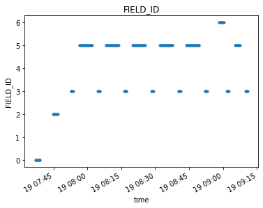
We can quickly spot check data fields using visplot. This is handy during subsequent analysis (although not intended for full scientific analysis).
The visplot function supports both standard x-y plots and x-y-c color mesh visualization. The mode is determined by the number of dimensions in the data passed in
[5]:
from cngi.dio import read_vis
from cngi.vis import visplot

# open a visibility xds
xds = read_vis('twhya.vis.zarr').xds0

# fields versus time coordinate
visplot(xds.FIELD_ID, axis='time')
overwrite_encoded_chunks True
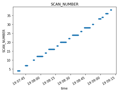
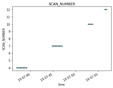
[6]:
visplot(xds.SCAN_NUMBER, 'time')
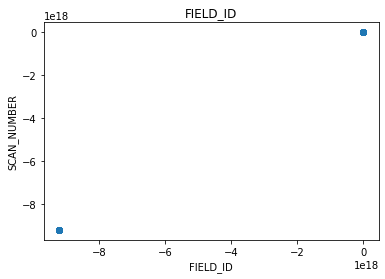
[7]:
# 2-D plot - fields versus scans
visplot(xds.FIELD_ID, xds.SCAN_NUMBER)
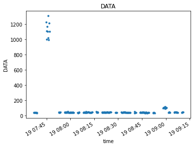
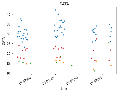
[8]:
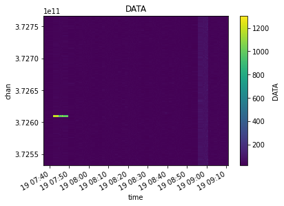
# 2-D plot of 4-D data - DATA over time
# when we specify an x-axis (time), the other axes (baseline, chan, pol) are averaged together
visplot(xds.DATA, axis='time')
[9]:
# 3-D plot of 4-D data - DATA over time and channel
# we can give two axes to create a color mesh visualization
visplot(xds.DATA, axis=['time','chan'])
Data Selection
The xarray Dataset format has extensive built-in functions for selecting data and splitting by different criteria. Often times the global data is referenced to identify particular values to select by.
Once the selection values are known, xds.isel(...) and xds.sel(...) can be used to select by dimension index or world value. xds.where(...) can be used to select by anything.
Lets start by examining the range of time and channel frequency values we have available in the visibility xds along with the field names and state ids in the global data.
[10]:
from cngi.dio import read_vis
import numpy as np

# open the master xds
mxds = read_vis('twhya.vis.zarr')

# inspect some properties
print('times: ', mxds.xds0.time.values[0], ' to ', mxds.xds0.time.values[-1])
print('chans: ', mxds.xds0.chan.values[0], ' to ', mxds.xds0.chan.values[-1])
print('fields: ', mxds.fields.values)
overwrite_encoded_chunks True
times:  2012-11-19T07:37:00.000000000  to  2012-11-19T09:11:01.631999969
chans:  372533086425.9812  to  372766851074.4187
fields:  ['J0522-364' 'J0539+145' 'Ceres' 'J1037-295' 'TW Hya' 'TW Hya' '3c279']
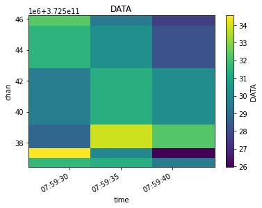
We can directly select specific dimension indices if we know what we’re looking for
[11]:
xds = mxds.xds0.isel(time=[76,77,78], chan=[6,7,8,12,20,21])

visplot(xds.DATA, ['time', 'chan'])
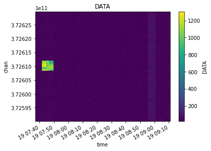
Or select by a range of dimension values, in this case lets select data between 372.59 and 372.63 GHz
[12]:
xds = mxds.xds0.sel(chan=slice(372.59e9, 372.63e9))

visplot(xds.DATA, ['time', 'chan'])
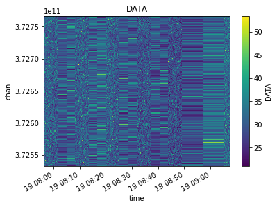
Or select by a particular field value, in this case lets select just the TW Hya fields
[13]:
fields = mxds.field_ids[np.where(mxds.fields == 'TW Hya')].values

xds = mxds.xds0.where(mxds.xds0.FIELD_ID.isin(fields), drop=True)

visplot(xds.DATA, axis=['time','chan'])
Finally, lets do a more complicated multi-selection
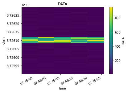
[14]:
xds = mxds.xds0.where(mxds.xds0.ANTENNA1.isin([2,3,4,5]) & mxds.xds0.ANTENNA2.isin([2,3,4,5]) &
                       (mxds.xds0.chan > 372.59e9) & (mxds.xds0.chan < 372.63e9) &
                       (mxds.xds0.time > np.datetime64('2012-11-19T07:45:50.0')) &
                       (mxds.xds0.time < np.datetime64('2012-11-19T07:46:30.0')),
                       drop=True)

visplot(xds.DATA, ['time', 'chan'])
Rather than cluttering each CNGI function with many parameters for data selection, instead the Dataset should be appropriately split before calling the relevant CNGI API function(s).
Splitting and Joining
Once you have the data selected that you want to work on, you can use split_dataset (was mstransform) to split that data out into its own mxds. The new mxds will include only the selected visibility and subtable data.
[15]:
from cngi.vis import split_dataset

# slice and split out the new mxds
xds_slice = mxds.xds0.sel(chan=slice(372.59e9, 372.63e9))
mxds_slice = mxds.assign_attrs(xds0=xds_slice) # replace xds0
mxds_slice = split_dataset(mxds_slice, 'xds0')

# we should now have a new mxds with less data, which we can see with a few print statements
print("Select a subset of channels. Unrelated data (such as antennas) to the remaining channels are dropped.")
print(f"old mxds: {len(mxds.xds0.chan)} chans, {len(mxds.antenna_ids)} antennas")
print(f"new mxds: {len(mxds_slice.xds0.chan)} chans, {len(mxds_slice.antenna_ids)} antennas")
Select a subset of channels. Unrelated data (such as antennas) to the remaining channels are dropped.
old mxds: 384 chans, 26 antennas
new mxds: 65 chans, 21 antennas
A split mxds, or several mxds gathered from different telescopes are times, can be merged back into a single mxds for further calibration or computation with join_dataset (was concat).
[16]:
from cngi.dio import read_vis
from cngi.vis import join_dataset
import numpy as np

# open the master xds
mxds = read_vis('twhya.vis.zarr')

# split out several channels to run computations on
mxds_slice0 = mxds.assign_attrs(xds0=mxds.xds0.sel(chan=slice(372.57e9, 372.60e9)))
mxds_slice1 = mxds.assign_attrs(xds0=mxds.xds0.sel(chan=slice(372.67e9, 372.70e9)))
# do channel-dependent operations...

# merge the split mxds into a single mxds (takes some time)
tmp_mxds = join_dataset(mxds_slice0, mxds_slice1) # mxds_slice1.xds0 is moved to mxds_cal.xds1
list(filter(lambda n: 'xds' in n, tmp_mxds.attrs.keys()))
overwrite_encoded_chunks True
Warning: reference value -1 in subtable WEATHER does not exist in ANTENNA.antenna_id!
Warning: reference value 5 in subtable FIELD does not exist in SOURCE.source_id!
[16]:
['xds0', 'xds1']
Similarly, visibilities can be merged with join_vis. Think really hard about when it is appropriate to use this function, however, since some meaning inherent to the data could be lost by doing further computation on the merged dataset.
[17]:
from cngi.vis import join_vis
from cngi.vis import visplot

# merge the slices back together
mxds_joined = join_vis(tmp_mxds, 'xds0', 'xds1')
visplot(mxds_joined.xds0.DATA, ['time', 'chan'])

# compare to the extra data in channels 372.60-372.62 which outshines everything
# xds_compare = mxds.xds0.sel(chan=slice(372.57e9, 372.70e9))
# visplot(xds_compare.DATA, ['time', 'chan'])
Flagging
Any boolean data variable can be used to flag any other data variable of common dimension(s).
Flagged values are set to np.nan, and subsequent math/analysis should be of the type that ignores nan values.
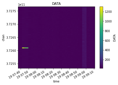
First lets see the original raw data
[18]:
from cngi.dio import read_vis

mxds = read_vis('twhya.vis.zarr')

visplot(mxds.xds0.DATA, ['time', 'chan'])
overwrite_encoded_chunks True
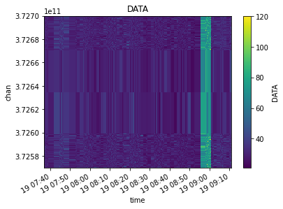
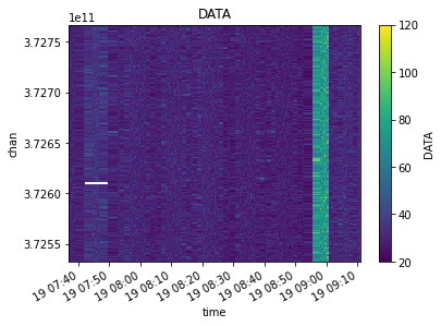
Now lets flag the entire dataset contents based on the value of the FLAG data variable. The bright line from Ceres is replaced with Nan’s (that appear as blank whitespace in the plot)
[19]:
from cngi.vis import apply_flags

flagged_xds = apply_flags(mxds, 'xds0', flags='FLAG')

visplot(flagged_xds.xds0.DATA, ['time', 'chan'])
Averaging and Smoothing
Averaging functions will change the shape of the resulting xarray dataset along the dimension being averaged.
Smoothing functions always return an xarray dataset with the same dimensions as the original.
We will use the TWHya dataset for this section. Dask may emit performance warnings if the chunk size is too small. We can increase our chunk size in the xds to any multiple of the chunk size used during conversion. We will do that here to avoid the performance warnings for this section. Note that baseline is already chunked at the maximum for its dimension size, so we can omit it.
[20]:
from cngi.dio import read_vis

mxds = read_vis('twhya.vis.zarr', chunks=({'time':200, 'chan':64, 'pol':2}))
overwrite_encoded_chunks True
Channel Averaging
The channel averaging function looks for all data variables in the dataset with a channel dimension and averages by the specified bin width. The returned dataset will have a different channel dimension size.
[21]:
from cngi.vis import chan_average, visplot
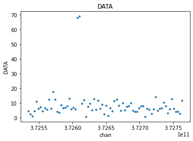
# average 5 channels of original unflagged data
avg_xds = chan_average(mxds, 'xds0', width=5)
# compare the original to the channel averaged
visplot(mxds.xds0.DATA[30,0,:,0], 'chan')
visplot(avg_xds.xds0.DATA[30,0,:,0], 'chan')
[22]:
# confirm new channel dimension after averaging
print(dict(mxds.xds0.dims))
print(dict(avg_xds.xds0.dims))
{'baseline': 210, 'chan': 384, 'pol': 2, 'pol_id': 1, 'spw_id': 1, 'time': 410, 'uvw_index': 3}
{'baseline': 210, 'chan': 76, 'pol': 2, 'pol_id': 1, 'spw_id': 1, 'time': 410, 'uvw_index': 3}
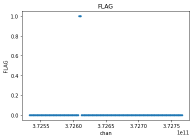
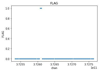
Since every variable with a channel dimension in the dataset is averaged, this will also include the FLAG variable. FLAG is a boolean type with values of 0 or 1 that are averaged over the width, resulting in a decimal number. The result is then typcast back to boolean, which is the same as just rounding up.
Long story short, if any channel in the width is flagged, the resulting averaged channel will also be flagged
[23]:
# compare the original flags to the channel averaged flags
visplot(mxds.xds0.FLAG[30,0,:,0], 'chan')
visplot(avg_xds.xds0.FLAG[30,0,:,0], 'chan')
One might want to apply flags before channel averaging
[24]:
from cngi.vis import apply_flags

flg_xds = apply_flags(mxds, 'xds0', flags=['FLAG'])
avg_flg_xds = chan_average(flg_xds, 'xds0', width=5)

visplot(flg_xds.xds0.DATA[30,0,:,0], 'chan')
visplot(avg_flg_xds.xds0.DATA[30,0,:,0], 'chan')
Or apply flags after channel averaging
[25]:
flg_avg_xds = apply_flags(avg_xds, 'xds0', flags=['FLAG'])

visplot(flg_avg_xds.xds0.DATA[30,0,:,0], 'chan')
There is a small difference of two points, made more clear when we overlay the plots
[26]:
visplot(avg_flg_xds.xds0.DATA[30,0,:,0], 'chan', drawplot=False)
visplot(flg_avg_xds.xds0.DATA[30,0,:,0], 'chan', overplot=True)
Time Averaging
The time averaging function can combine adjacent time steps or resample to a new uniform time step. This affects all fields in the xds that have a time dimension. The span parameter can be used to limit averaging to just the time steps within each scan, or within each state. The returned dataset will have a different time dimension size.
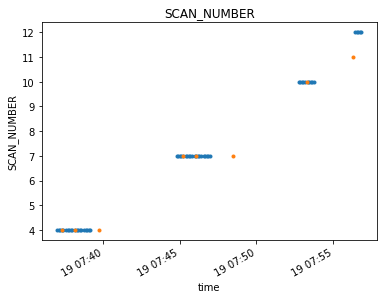
First let’s average across the states in a scan using a bin of 7
[27]:
from cngi.vis import time_average

state_xds = time_average(mxds,'xds0', bin=7, span='state')

visplot(mxds.xds0.SCAN_NUMBER.where(mxds.xds0.time < np.datetime64('2012-11-19T07:57:00.0'), drop=True), 'time', drawplot=False)
visplot(state_xds.xds0.SCAN_NUMBER.where(state_xds.xds0.time < np.datetime64('2012-11-19T07:57:00.0'), drop=True), 'time', overplot=True)
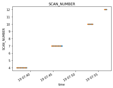
Averaging across both state and scan allows the bins to cross the time gaps between scans.
[28]:
both_xds = time_average(mxds, 'xds0', bin=7, span='both')

visplot(mxds.xds0.SCAN_NUMBER.where(mxds.xds0.time < np.datetime64('2012-11-19T07:57:00.0'), drop=True), 'time', drawplot=False)
visplot(both_xds.xds0.SCAN_NUMBER.where(both_xds.xds0.time < np.datetime64('2012-11-19T07:57:00.0'), drop=True), 'time', overplot=True)
Switching to the width parameter will resample the contents of the xds to a uniform time bin across the span
[29]:
resampled_xds = time_average(mxds, 'xds0', width='20s', span='state')

visplot(mxds.xds0.SCAN_NUMBER.where(mxds.xds0.time < np.datetime64('2012-11-19T07:57:00.0'), drop=True), 'time', drawplot=False)
visplot(resampled_xds.xds0.SCAN_NUMBER.where(resampled_xds.xds0.time < np.datetime64('2012-11-19T07:57:00.0'), drop=True), 'time', overplot=True)
In all cases, the dimensionality of the time averaged xds returned will be different than the start.
[30]:
print(dict(mxds.xds0.dims))
print(dict(state_xds.xds0.dims))
print(dict(both_xds.xds0.dims))
print(dict(resampled_xds.xds0.dims))
{'baseline': 210, 'chan': 384, 'pol': 2, 'pol_id': 1, 'spw_id': 1, 'time': 410, 'uvw_index': 3}
{'baseline': 210, 'chan': 384, 'pol': 2, 'pol_id': 1, 'spw_id': 1, 'time': 68, 'uvw_index': 3}
{'baseline': 210, 'chan': 384, 'pol': 2, 'pol_id': 1, 'spw_id': 1, 'time': 59, 'uvw_index': 3}
{'baseline': 210, 'chan': 384, 'pol': 2, 'pol_id': 1, 'spw_id': 1, 'time': 150, 'uvw_index': 3}
We can inspect the affect of different time averaging methods on the DATA contents
[31]:
timefilter = np.datetime64('2012-11-19T07:57:00.0')
visplot(mxds.xds0.DATA.where(mxds.xds0.time < timefilter, drop=True)[:,:,100,0], 'time', drawplot=False)
visplot(state_xds.xds0.DATA.where(state_xds.xds0.time < timefilter, drop=True)[:,:,100,0], 'time', overplot=True, drawplot=False)
visplot(both_xds.xds0.DATA.where(both_xds.xds0.time < timefilter, drop=True)[:,:,100,0], 'time', overplot=True, drawplot=False)
visplot(resampled_xds.xds0.DATA.where(resampled_xds.xds0.time < timefilter, drop=True)[:,:,100,0], 'time', overplot=True)
Flagging works the same way as in channel averaging. Flags are averaged with all other data sharing the time axis. They may be applied before or after time averaging. The time averaged flag field is converted back to boolean. Any single flagged value in the original data will cause the entire bin to be flagged in the resulting data.
Channel Smoothing
Channel smoothing allows a variety of window shapes to be convolved across the channel dimension to smooth over changes from bin to bin. The standard CASA hanning smooth is supported as the default option. The returned dataset will have the same dimensions as the original.
[32]:
from cngi.vis import chan_smooth

smooth_xds = chan_smooth(mxds, 'xds0')

visplot(mxds.xds0.DATA[30,0,:,0], 'chan', drawplot=False)
visplot(smooth_xds.xds0.DATA[30,0,:,0], 'chan', overplot=True)
chansmooth uses the scipy.signal package to set the window shape. Therefore, all the window functions supported by scipy are also supported here. The size of the window width is configurable.
https://docs.scipy.org/doc/scipy/reference/signal.windows.html#module-scipy.signal.windows
[33]:
bohman_xds = chan_smooth(mxds, 'xds0', type='bohman', size=7)

visplot(smooth_xds.xds0.DATA[30,0,:,0], 'chan', drawplot=False)
visplot(bohman_xds.xds0.DATA[30,0,:,0], 'chan', overplot=True)
non-unity gains are also supported to amplify or attenuate the output
[34]:
hann_xds = chan_smooth(mxds, 'xds0', type='hann', size=5, gain=1.0)
amp_hann_xds = chan_smooth(mxds, 'xds0', type='hann', size=5, gain=3.0)

visplot(hann_xds.xds0.DATA[30,0,:,0], 'chan', drawplot=False)
visplot(amp_hann_xds.xds0.DATA[30,0,:,0], 'chan', overplot=True)
UV Fitting
Various modeling can be performed in the UV-domain through polynomial regression on the visibility data.
The uvcontfit function takes a source data variable in the xarray dataset and fits a polynomial of fitorder across the channel axis. The resulting model is placed in the target data variable and retains the dimensionality of the source. Specified channels may be excluded to focus on fitting only continuum visibilities and not line emissions.
In our example dataset we know that the Ceres has a line emission, so let’s focus on just that field. We will need to master xarray dataset to see which field ID(s) is Ceres.
[35]:
from cngi.dio import read_vis
from cngi.vis import uv_cont_fit, visplot
import dask.config
dask.config.set({"array.slicing.split_large_chunks": False})

mxds = read_vis('twhya.vis.zarr')

fields = mxds.field_ids[np.where(mxds.fields == 'Ceres')].values

mxds = mxds.assign_attrs({'ceres_xds':mxds.xds0.where(mxds.xds0.FIELD_ID.isin(fields), drop=True)})

fit_xds = uv_cont_fit(mxds, 'ceres_xds', source='DATA', target='CONTFIT')

visplot(fit_xds.ceres_xds.DATA, ['time', 'chan'])
visplot(fit_xds.ceres_xds.CONTFIT, ['time', 'chan'])
overwrite_encoded_chunks True
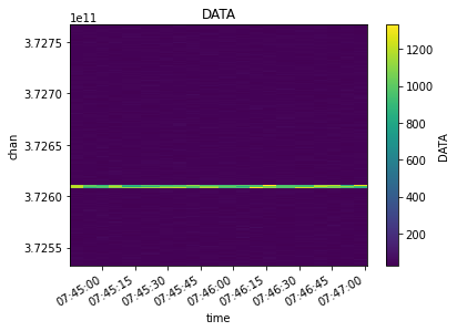
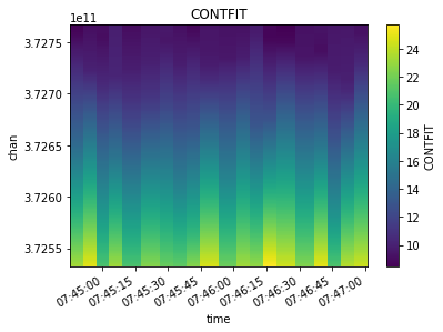
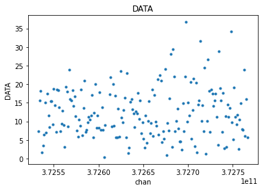
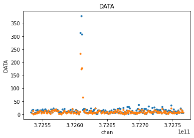
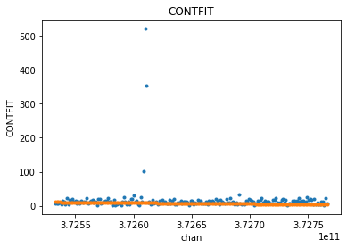
What we are seeing is merged across baselines and polarizations. Let’s look at just one time/baseline/pol sample and examine the fit. The linear fit is skewed by the line emission towards one side of the channel axis.
[36]:
visplot(fit_xds.ceres_xds.DATA[10,10,:,0], ['chan'], drawplot=False)
visplot(fit_xds.ceres_xds.CONTFIT[10,10,:,0], ['chan'], overplot=True)
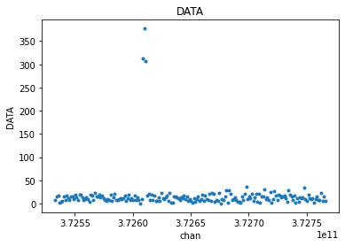
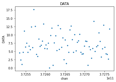
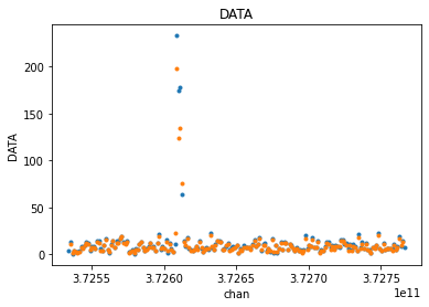
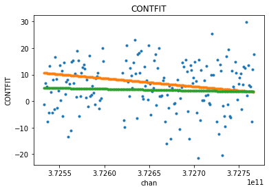
Let’s omit the channels with the line emission and do the fit again. We should see less skewing in the fitted continuum.
The fits appear lower in value than the mean of the data when viewing the magnitude of complex visibilities. The real and imaginary parts are fitted individually. We examine just the real piece here to see a that the fit is indeed a decent approximation through the center of the data.
[37]:
excludechans = np.where( (mxds.xds0.chan > 3.726e11) & (mxds.xds0.chan < 3.7262e11) )[0]

fit_xds2 = uv_cont_fit(mxds, 'ceres_xds', source='DATA', target='CONTFIT', fitorder=1, excludechans=excludechans)

includechans = np.setdiff1d( range(mxds.xds0.dims['chan']), excludechans)
visplot(fit_xds2.ceres_xds.DATA[10,10,includechans,0].real, ['chan'], drawplot=False)
visplot(fit_xds.ceres_xds.CONTFIT[10,10,:,0].real, ['chan'], drawplot=False, overplot=True)
visplot(fit_xds2.ceres_xds.CONTFIT[10,10,:,0].real, ['chan'], overplot=True)
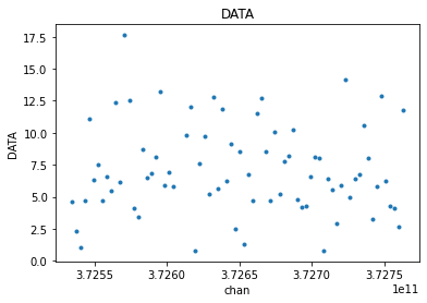
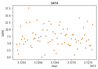
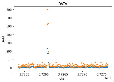
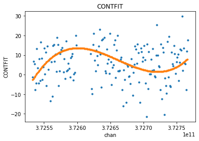
For even more fun, we can try a higher order fit. Let’s use all channels to allow the line emission to exaggerate the non-linearity, but only plot the continuum DATA channels so the y-scale stays smaller.
[38]:
fit_xds3 = uv_cont_fit(mxds, 'ceres_xds', source='DATA', target='CONTFIT', fitorder=3, excludechans=[])

visplot(fit_xds3.ceres_xds.DATA[10,10,includechans,0].real, ['chan'], drawplot=False)
visplot(fit_xds3.ceres_xds.CONTFIT[10,10,:,0].real, ['chan'], overplot=True)
Several metrics related to the quality of the fit are stored in the xarray dataset attributes section as metadata. They are named with a prefix matching the target parameter in uvcontfit.
[39]:
metrics = [kk for kk in fit_xds.ceres_xds.attrs.keys() if kk.startswith('CONTFIT')]
print(metrics)

print(fit_xds.ceres_xds.CONTFIT_rms_error)
['CONTFIT_rms_error', 'CONTFIT_min_max_error', 'CONTFIT_bw_frac', 'CONTFIT_freq_frac']
<xarray.DataArray ()>
dask.array<pow, shape=(), dtype=complex128, chunksize=(), chunktype=numpy.ndarray>
One thing to note is that these metrics are dask elements, and are not actually computed until explicity requested. Things like visplot explicity force the computation of the data needed for plotting, but nothing has forced these metrics to be computed yet. So we will call .compute() to see their values.
[40]:
print('rms error with line included: ', fit_xds.ceres_xds.CONTFIT_rms_error.values)
print('rms error with line excluded: ', fit_xds2.ceres_xds.CONTFIT_rms_error.values)
rms error with line included:  (16.444908051664182-0.7566763926282181j)
rms error with line excluded:  (0.37306136672597817-0.007993456030923675j)